Clustering Metrics

Loading Packages

import warnings
warnings.filterwarnings('ignore')

import matplotlib.pyplot as plt
from matplotlib.patches import Patch
import pandas as pd
import numpy as np
import scanpy as sc
from sklearn.metrics import adjusted_rand_score, adjusted_mutual_info_score, normalized_mutual_info_score

Loading Data

## results for three methods under different noise levels
adata_results_noised = sc.read_h5ad("../../../Mouse_Thymus_Noised.h5ad")
print(adata_results_noised)

## original results
adata_results = sc.read_h5ad("../../../Mouse_Thymus_Replicate1.h5ad")
print(adata_results)

AnnData object with n_obs × n_vars = 4183 × 0
    obs: 'SpatialGlue_level_1', 'SpatialGlue_level_2', 'SpatialGlue_level_3', 'SpatialCOC_level_1', 'SpatialCOC_level_2', 'SpatialCOC_level_3', 'MultiMAP_level_1', 'MultiMAP_level_2', 'MultiMAP_level_3'
    uns: 'MultiMAP_level_1_colors', 'MultiMAP_level_2_colors', 'MultiMAP_level_3_colors', 'SpaKnit_level_1_colors', 'SpaKnit_level_2_colors', 'SpaKnit_level_3_colors', 'SpatialGlue_level_1_colors', 'SpatialGlue_level_2_colors', 'SpatialGlue_level_3_colors'
    obsm: 'spatial'
AnnData object with n_obs × n_vars = 4183 × 0
    obs: 'SpatialCOC', 'SpatialGlue', 'STAGATE', 'Modality1', 'Modality2', 'SpaGCN', 'MultiMAP', 'MultiVI', 'Seurat', 'COSMOS'
    obsm: 'COSMOS', 'Modality1', 'Modality2', 'MultiMAP', 'MultiVI', 'STAGATE', 'Seurat', 'SpatialCOC', 'SpatialGlue', 'spatial'

Calculating Metrics

methods = ['SpatialCOC', 'SpatialGlue', 'MultiMAP']
levels = ['level_1', 'level_2', 'level_3']

# 初始化结果存储
results = []

# 遍历每种方法和层次
for method in methods:
    for level in levels:
        # 提取真实标签和预测标签
        true_labels = adata_results.obs[method]  # 真实标签
        pred_labels = adata_results_noised.obs[f"{method}_{level}"]  # 预测标签

        # 计算指标
        ari = adjusted_rand_score(true_labels, pred_labels)
        ami = adjusted_mutual_info_score(true_labels, pred_labels)
        nmi = normalized_mutual_info_score(true_labels, pred_labels)

        # 存储结果
        results.append({
            'Method': method,
            'Noise Level': level,
            'ARI': ari,
            'AMI': ami,
            'NMI': nmi
        })

# 将结果转换为DataFrame
results_df = pd.DataFrame(results)

# 打印结果
print(results_df)

results_df.to_excel('Robustness.xlsx', index=False, engine='openpyxl')

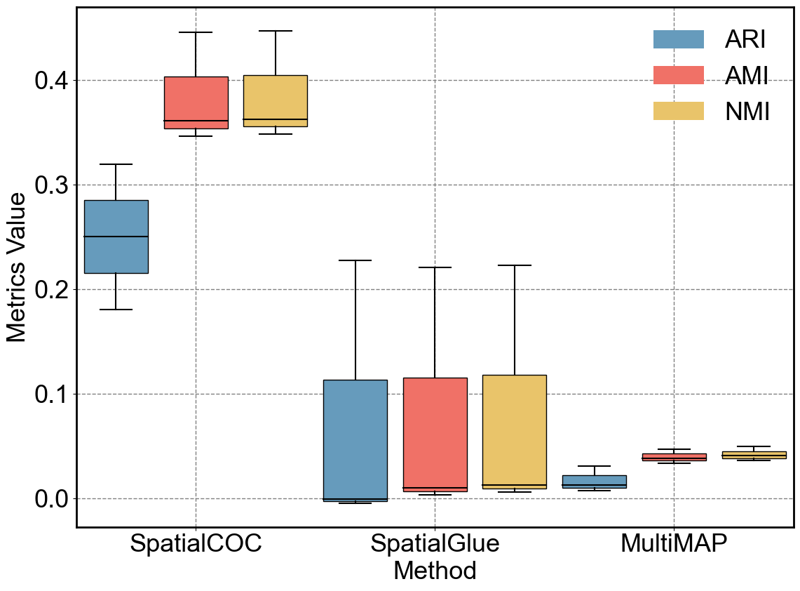
        Method Noise Level       ARI       AMI       NMI
0   SpatialCOC     level_1  0.319763  0.446140  0.447533
1   SpatialCOC     level_2  0.180623  0.346918  0.348702
2   SpatialCOC     level_3  0.250694  0.361333  0.362970
3  SpatialGlue     level_1  0.227981  0.220949  0.223135
4  SpatialGlue     level_2 -0.004561  0.010486  0.013236
5  SpatialGlue     level_3 -0.000556  0.003481  0.006076
6     MultiMAP     level_1  0.030888  0.047189  0.049527
7     MultiMAP     level_2  0.013195  0.033981  0.036472
8     MultiMAP     level_3  0.007821  0.038593  0.041075

# Organize the data for plotting
metrics_results = results_df.pivot(index='Method', columns='Level', values=['ARI', 'AMI', 'NMI'])
metrics_results.columns = [f"{metric}_{level}" for metric, level in metrics_results.columns]

# Extract the data
box_data = []
methods = ['SpaKnit', 'SpatialGlue', 'MultiMAP']  # Ensure the order of methods
for method in methods:
    for metric in ['ARI', 'AMI', 'NMI']:
        box_data.append([metrics_results.loc[method, f"{metric}_{level}"] for level in levels])

Ploting

# Set the font size and font family for matplotlib
plt.rcParams.update({'font.size': 26, 'font.family': 'Arial'})
box_width = 0.8

# Create the boxplot
fig, ax = plt.subplots(figsize=(12, 9))
box = ax.boxplot(box_data, patch_artist=True, widths=box_width)

# Customize the style of the boxplot elements
for element in ['whiskers', 'caps', 'medians']:
    for elem in box[element]:
        elem.set_color('black')
        elem.set_linewidth(1.5)

# Set the colors for the boxes
colors = ['#669bbc', '#f07167', '#e9c46a'] * len(methods)
for patch, color in zip(box['boxes'], colors):
    patch.set_facecolor(color)

# Set the x-axis tick labels
num_methods = len(methods)
num_metrics = 3
tick_positions = np.arange(2, num_methods * num_metrics + 1, num_metrics)
ax.set_xticks(tick_positions)
ax.set_xticklabels(['SpatialCOC', 'SpatialGlue', 'MultiMAP'])

plt.title('')  # Empty title
plt.xlabel('Method')
plt.ylabel('Metrics Value')

# Customize the thickness of the plot's border
for spine in plt.gca().spines.values():
    spine.set_linewidth(2)

plt.grid(True, linestyle='--', color='gray', linewidth=1)

# Add the legend
legend_elements = [Patch(facecolor='#669bbc', label='ARI'),
                   Patch(facecolor='#f07167', label='AMI'),
                   Patch(facecolor='#e9c46a', label='NMI')]
ax.legend(handles=legend_elements, loc='upper right', frameon=False)

plt.tight_layout()

# Save the plot as PNG and EPS files
plt.savefig('Metrics of Three Methods.png', dpi=500)
plt.savefig('Metrics of Three Methods.eps')

plt.show()